
Analyzing gender bias in movie dialogues
In this post, I’ve tried to analyze gender bias in Hollywood movies using the character dialogues & some movie metadata. The gender bias can be established if we can predict the gender of a Hollywood movie character based on his / her dialogues in the movie. The dataset was released by Cornell University. The data pre-processing, EDA & modeling are all done in Python3 in a Jupyter notebook environment, rendered finally into a Markdown for this blog.
Import necessary libraries
import pandas as pd
import numpy as np
import re
from nltk.corpus import stopwords
from nltk.stem import WordNetLemmatizer
from wordcloud import WordCloud
import matplotlib.pyplot as plt
import seaborn as sns
import warnings

from sklearn.preprocessing import OneHotEncoder, StandardScaler, MinMaxScaler
from sklearn.compose import ColumnTransformer
from sklearn.feature_extraction.text import TfidfTransformer, CountVectorizer, TfidfVectorizer
from sklearn.preprocessing import FunctionTransformer
from sklearn.linear_model import LogisticRegression
from sklearn.naive_bayes import MultinomialNB
from sklearn.ensemble import RandomForestClassifier,BaggingClassifier
from sklearn.svm import SVC
from sklearn.calibration import CalibratedClassifierCV
from sklearn.metrics import classification_report, confusion_matrix
from sklearn.pipeline import FeatureUnion, Pipeline
from sklearn.model_selection import train_test_split
from sklearn.base import BaseEstimator, TransformerMixin
from sklearn import svm
from sklearn.multiclass import OneVsRestClassifier
from sklearn.svm import LinearSVC

from imblearn.under_sampling import RandomUnderSampler
import eli5

import IPython
from IPython.display import display
import graphviz
from sklearn.tree import export_graphviz
import re


warnings.filterwarnings('ignore')
pd.set_option('display.max_rows', 100)
/opt/conda/lib/python3.7/site-packages/sklearn/utils/deprecation.py:143: FutureWarning: The sklearn.metrics.scorer module is  deprecated in version 0.22 and will be removed in version 0.24. The corresponding classes / functions should instead be imported from sklearn.metrics. Anything that cannot be imported from sklearn.metrics is now part of the private API.
  warnings.warn(message, FutureWarning)
/opt/conda/lib/python3.7/site-packages/sklearn/utils/deprecation.py:143: FutureWarning: The sklearn.feature_selection.base module is  deprecated in version 0.22 and will be removed in version 0.24. The corresponding classes / functions should instead be imported from sklearn.feature_selection. Anything that cannot be imported from sklearn.feature_selection is now part of the private API.
  warnings.warn(message, FutureWarning)
Reading the dataset
lines_df = pd.read_csv('../input/movie_lines.tsv', sep='\t', error_bad_lines=False,
                       warn_bad_lines=False, header=None)
characters_df = pd.read_csv('../input/movie_characters_metadata.tsv', sep='\t',
                            warn_bad_lines=False, error_bad_lines=False, header=None)

characters_df.head()
| 0 | 1 | 2 | 3 | 4 | 5 | |
|---|---|---|---|---|---|---|
| 0 | u0 | BIANCA | m0 | 10 things i hate about you | f | 4 |
| 1 | u1 | BRUCE | m0 | 10 things i hate about you | ? | ? |
| 2 | u2 | CAMERON | m0 | 10 things i hate about you | m | 3 |
| 3 | u3 | CHASTITY | m0 | 10 things i hate about you | ? | ? |
| 4 | u4 | JOEY | m0 | 10 things i hate about you | m | 6 |
Adding column names to characters dataframe
characters_df.columns=['chId','chName','mId','mName','gender','posCredits']
characters_df.head()
| chId | chName | mId | mName | gender | posCredits | |
|---|---|---|---|---|---|---|
| 0 | u0 | BIANCA | m0 | 10 things i hate about you | f | 4 |
| 1 | u1 | BRUCE | m0 | 10 things i hate about you | ? | ? |
| 2 | u2 | CAMERON | m0 | 10 things i hate about you | m | 3 |
| 3 | u3 | CHASTITY | m0 | 10 things i hate about you | ? | ? |
| 4 | u4 | JOEY | m0 | 10 things i hate about you | m | 6 |
characters_df.shape
(9034, 6)
Checking the distribution of gender in the characters dataset
characters_df.gender.value_counts()
?    6008
m    1899
f     921
M     145
F      44
Name: gender, dtype: int64
We need to clean this column. Let’s also remove the characters where gender information is not available. We’ll assign a label of 0 to male characters & 1 to female characters.
characters_df = characters_df[characters_df.gender != '?']
characters_df.gender = characters_df.gender.apply(lambda g: 0 if g in ['m', 'M'] else 1)  ## Label encoding

characters_df.shape
(3026, 6)
characters_df.gender.value_counts()
0    2044
1     982
Name: gender, dtype: int64
Let’s also take a look at the position of the character in the post credits of the movie
characters_df.posCredits.value_counts()
1       497
2       443
3       352
?       330
4       268
5       211
6       169
7       125
8       100
9        79
10       54
11       40
1000     38
13       33
12       32
16       26
14       24
18       24
17       19
19       18
15       14
21       13
22        9
20        8
29        7
27        6
24        5
25        5
26        5
45        4
23        4
31        4
35        4
38        3
43        3
33        3
34        3
36        2
59        2
39        2
30        2
42        2
28        2
32        2
51        1
82        1
44        1
70        1
46        1
41        1
63        1
37        1
50        1
49        1
47        1
62        1
71        1
Name: posCredits, dtype: int64
The position of characters in the credits section seems to be a useful feature for classification. We can try to use it as a categorical variable later. But let’s combine the low frequency ones together first.
characters_df.posCredits = characters_df.posCredits.apply(lambda p: '10+' if not p in ['1', '2', '3', '4', '5', '6', '7', '8', '9'] else p)  ## Label encoding
characters_df.posCredits.value_counts()
10+    782
1      497
2      443
3      352
4      268
5      211
6      169
7      125
8      100
9       79
Name: posCredits, dtype: int64
Let’s clean the lines dataframe now!
lines_df.columns = ['lineId','chId','mId','chName','dialogue']
lines_df.head()
| lineId | chId | mId | chName | dialogue | |
|---|---|---|---|---|---|
| 0 | L1045 | u0 | m0 | BIANCA | They do not! |
| 1 | L1044 | u2 | m0 | CAMERON | They do to! |
| 2 | L985 | u0 | m0 | BIANCA | I hope so. |
| 3 | L984 | u2 | m0 | CAMERON | She okay? |
| 4 | L925 | u0 | m0 | BIANCA | Let's go. |
Let’s join lines_df and characters_df together.
df = pd.merge(lines_df, characters_df, how='inner', on=['chId','mId', 'chName'],
         left_index=False, right_index=False, sort=True,
         copy=False, indicator=False)
df.head()
| lineId | chId | mId | chName | dialogue | mName | gender | posCredits | |
|---|---|---|---|---|---|---|---|---|
| 0 | L1045 | u0 | m0 | BIANCA | They do not! | 10 things i hate about you | 1 | 4 |
| 1 | L985 | u0 | m0 | BIANCA | I hope so. | 10 things i hate about you | 1 | 4 |
| 2 | L925 | u0 | m0 | BIANCA | Let's go. | 10 things i hate about you | 1 | 4 |
| 3 | L872 | u0 | m0 | BIANCA | Okay -- you're gonna need to learn how to lie. | 10 things i hate about you | 1 | 4 |
| 4 | L869 | u0 | m0 | BIANCA | Like my fear of wearing pastels? | 10 things i hate about you | 1 | 4 |
df.shape
(229309, 8)
Remove empty dialogues from the dataset
df = df[df['dialogue'].notnull()]
df.shape
(229106, 8)
Let’s check what kind of movie metadata we can add to our dataset.
movies = pd.read_csv("../input/movie_titles_metadata.tsv", sep='\t', error_bad_lines=False,
                       warn_bad_lines=False, header=None)
movies.columns = ['mId','mName','releaseYear','rating','votes','genres']

movies.head()
| mId | mName | releaseYear | rating | votes | genres | |
|---|---|---|---|---|---|---|
| 0 | m0 | 10 things i hate about you | 1999 | 6.9 | 62847.0 | ['comedy' 'romance'] |
| 1 | m1 | 1492: conquest of paradise | 1992 | 6.2 | 10421.0 | ['adventure' 'biography' 'drama' 'history'] |
| 2 | m2 | 15 minutes | 2001 | 6.1 | 25854.0 | ['action' 'crime' 'drama' 'thriller'] |
| 3 | m3 | 2001: a space odyssey | 1968 | 8.4 | 163227.0 | ['adventure' 'mystery' 'sci-fi'] |
| 4 | m4 | 48 hrs. | 1982 | 6.9 | 22289.0 | ['action' 'comedy' 'crime' 'drama' 'thriller'] |
movie_yr = movies[['mId', 'releaseYear']]
movie_yr.releaseYear = pd.to_numeric(movie_yr.releaseYear.apply(lambda y: str(y)[0:4]), errors='coerce')
movie_yr = movie_yr.dropna()
We will just add the year of movie release to our dataset.
df = pd.merge(df, movie_yr, how='inner', on=['mId'],
         left_index=False, right_index=False, sort=True,
         copy=False, indicator=False)
df.head()
| lineId | chId | mId | chName | dialogue | mName | gender | posCredits | releaseYear | |
|---|---|---|---|---|---|---|---|---|---|
| 0 | L1045 | u0 | m0 | BIANCA | They do not! | 10 things i hate about you | 1 | 4 | 1999.0 |
| 1 | L985 | u0 | m0 | BIANCA | I hope so. | 10 things i hate about you | 1 | 4 | 1999.0 |
| 2 | L925 | u0 | m0 | BIANCA | Let's go. | 10 things i hate about you | 1 | 4 | 1999.0 |
| 3 | L872 | u0 | m0 | BIANCA | Okay -- you're gonna need to learn how to lie. | 10 things i hate about you | 1 | 4 | 1999.0 |
| 4 | L869 | u0 | m0 | BIANCA | Like my fear of wearing pastels? | 10 things i hate about you | 1 | 4 | 1999.0 |
Feature Engineering
- Length of lines
- Count of lines
- One hot encodings for tokens
df['lineLength'] = df.dialogue.str.len()             ## Length of each line by characters
df['wordCountLine'] = df.dialogue.str.count(' ') + 1 ## Length of each line by words
df.head()
| lineId | chId | mId | chName | dialogue | mName | gender | posCredits | releaseYear | lineLength | wordCountLine | |
|---|---|---|---|---|---|---|---|---|---|---|---|
| 0 | L1045 | u0 | m0 | BIANCA | They do not! | 10 things i hate about you | 1 | 4 | 1999.0 | 12 | 3 |
| 1 | L985 | u0 | m0 | BIANCA | I hope so. | 10 things i hate about you | 1 | 4 | 1999.0 | 10 | 3 |
| 2 | L925 | u0 | m0 | BIANCA | Let's go. | 10 things i hate about you | 1 | 4 | 1999.0 | 9 | 2 |
| 3 | L872 | u0 | m0 | BIANCA | Okay -- you're gonna need to learn how to lie. | 10 things i hate about you | 1 | 4 | 1999.0 | 46 | 10 |
| 4 | L869 | u0 | m0 | BIANCA | Like my fear of wearing pastels? | 10 things i hate about you | 1 | 4 | 1999.0 | 32 | 6 |
Next, let’s convert the dialogues into clean tokens
- Remove Stopwords : because they occur very often, but serve no meaning. For eg. : is,am,are,the.
- Turn all word to smaller cases : I, i -> i
- Lemmatization: convert words to their root form. For eg., walk,walks -> walk or geographical,geographic -> geographic
wordnet_lemmatizer = WordNetLemmatizer()
def clean_dialogue( dialogue ):
    # Function to convert a raw review to a string of words
    # The input is a single string (a raw movie review), and
    # the output is a single string (a preprocessed movie review)
    # Source : https://www.kaggle.com/akerlyn/wordcloud-based-on-character
    #
    # 1. Remove HTML
    #
    # 2. Remove non-letters
    letters_only = re.sub("[^a-zA-Z]", " ", dialogue)
    #
    # 3. Convert to lower case, split into individual words
    words = letters_only.lower().split()
    #
    # 4. In Python, searching a set is much faster than searching
    #   a list, so convert the stop words to a set
    stops = set(stopwords.words("english"))

    # 5. Use lemmatization and remove stop words
    meaningful_words = [wordnet_lemmatizer.lemmatize(w) for w in words if not w in stops]
    #
    # 6. Join the words back into one string separated by space,
    # and return the result.
    return( " ".join( meaningful_words ))

df['cleaned_dialogue'] = df['dialogue'].apply(clean_dialogue)
df[['dialogue','cleaned_dialogue']].sample(5)
| dialogue | cleaned_dialogue | |
|---|---|---|
| 14684 | Thank you. | thank |
| 58592 | Hi tough guy. I guess it worked huh? | hi tough guy guess worked huh |
| 209279 | I've decided not to open a practice here I wa... | decided open practice want set research clinic... |
| 95420 | Am I suppose to be this sore? | suppose sore |
| 50378 | You could still always give Becker an itch. 'C... | could still always give becker itch course mig... |
Create training dataset
Now, we can aggregate all data for a particular movie character into 1 record. We will combine their dialogue tokens from the entire movie, calculate their median dialogue length by characters & words, and count their total no of lines in the movie.
train = df.groupby(['chId', 'mId', 'chName', 'gender', 'posCredits','releaseYear']). \
            agg({'lineLength' : ['median'],
                 'wordCountLine' : ['median'],
                 'chId' : ['count'],
                 'cleaned_dialogue' : [lambda x : ' '.join(x)]
                })

## Renaming columns by aggregate functions
train.columns = ["_".join(x) for x in train.columns.ravel()]

train.reset_index(inplace=True)
train
| chId | mId | chName | gender | posCredits | releaseYear | lineLength_median | wordCountLine_median | chId_count | cleaned_dialogue_<lambda> | |
|---|---|---|---|---|---|---|---|---|---|---|
| 0 | u0 | m0 | BIANCA | 1 | 4 | 1999.0 | 34.0 | 7.0 | 94 | hope let go okay gonna need learn lie like fe... |
| 1 | u100 | m6 | AMY | 1 | 7 | 1999.0 | 23.0 | 4.0 | 31 | died sleep three day ago paper tom dead calli... |
| 2 | u1003 | m65 | RICHARD | 0 | 3 | 1996.0 | 24.5 | 5.0 | 70 | asked would said room room serious foolin arou... |
| 3 | u1005 | m65 | SETH | 0 | 2 | 1996.0 | 37.0 | 8.0 | 163 | let follow said new jesus christ carlos brothe... |
| 4 | u1008 | m66 | C.O. | 0 | 10+ | 1997.0 | 48.0 | 9.0 | 33 | course uh v p security arrangement generally t... |
| ... | ... | ... | ... | ... | ... | ... | ... | ... | ... | ... |
| 2946 | u980 | m63 | VICTOR | 0 | 3 | 1931.0 | 32.0 | 6.0 | 126 | never said name remembers kill draw line take... |
| 2947 | u983 | m64 | ALICE | 1 | 10+ | 2009.0 | 30.0 | 6.0 | 51 | maybe wait mr christy killer still bill bill b... |
| 2948 | u985 | m64 | BILL | 0 | 10+ | 2009.0 | 20.0 | 4.0 | 39 | twenty mile crossroad steve back hour thing st... |
| 2949 | u997 | m65 | JACOB | 0 | 1 | 1996.0 | 36.0 | 6.0 | 90 | meant son daughter oh daughter bathroom vacati... |
| 2950 | u998 | m65 | KATE | 1 | 4 | 1996.0 | 20.0 | 4.5 | 44 | everybody go home going em swear god father ch... |
2951 rows × 10 columns
Let’s check some feature distributions by gender
sns.boxplot(data = train, x = 'gender', y = 'chId_count', hue = 'gender')
<matplotlib.axes._subplots.AxesSubplot at 0x7fe92d3d57d0>
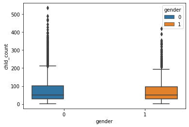
The chId_count here refers to the no of lines given to the character in the movie. While the median value seems to be roughly similar for both males & females, the upper bound seems to be higher for males.
sns.boxplot(data = train, x = 'gender', y = 'wordCountLine_median', hue = 'gender')
<matplotlib.axes._subplots.AxesSubplot at 0x7fe92d108550>
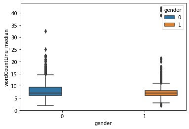
The count of words per dialogue is higher for male characters than that for female characters!
sns.boxplot(data = train, x = 'gender', y = 'lineLength_median', hue = 'gender')
<matplotlib.axes._subplots.AxesSubplot at 0x7fe92d0a1dd0>
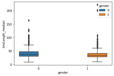
The median length of a dialogue also seems to be higher for males.
sns.scatterplot(data = train, x = 'wordCountLine_median', y = 'chId_count', hue = 'gender', alpha = 0.5)
<matplotlib.axes._subplots.AxesSubplot at 0x7fe93902b810>
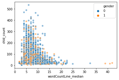
Again, in the scatter plot, we see female characters, ie yellow points, generally closer to the origin, as they have smaller dialogues & lesser dialogues per movie, while male characters denoted by blue dots are more outward from the origin.
Train test split
Now, we can split our data into a training set & a validation set.
## Separating labels from features
y = train['gender']
X = train.copy()
X.drop('gender', axis=1, inplace=True)

## Removing unnecessary columns
X.drop('chId', axis=1, inplace=True)
X.drop('mId', axis=1, inplace=True)
X.drop('chName', axis=1, inplace=True)
X.head()
| posCredits | releaseYear | lineLength_median | wordCountLine_median | chId_count | cleaned_dialogue_<lambda> | |
|---|---|---|---|---|---|---|
| 0 | 4 | 1999.0 | 34.0 | 7.0 | 94 | hope let go okay gonna need learn lie like fe... |
| 1 | 7 | 1999.0 | 23.0 | 4.0 | 31 | died sleep three day ago paper tom dead calli... |
| 2 | 3 | 1996.0 | 24.5 | 5.0 | 70 | asked would said room room serious foolin arou... |
| 3 | 2 | 1996.0 | 37.0 | 8.0 | 163 | let follow said new jesus christ carlos brothe... |
| 4 | 10+ | 1997.0 | 48.0 | 9.0 | 33 | course uh v p security arrangement generally t... |
We will pick equal no of records for both male & female characters to avoid any kind of bias due to no of records.
undersample = RandomUnderSampler(sampling_strategy='majority')
X_under, y_under = undersample.fit_resample(X, y)
y_under.value_counts()
1    948
0    948
Name: gender, dtype: int64
We’ll also try to keep equal no of male & female records in the train & validation datasets
X_train, X_val, y_train, y_val = train_test_split(X_under, y_under, test_size=0.2, random_state = 10, stratify=y_under)

y_val.value_counts()
1    190
0    190
Name: gender, dtype: int64
X_val.head()
| posCredits | releaseYear | lineLength_median | wordCountLine_median | chId_count | cleaned_dialogue_<lambda> | |
|---|---|---|---|---|---|---|
| 1236 | 2 | 2001.0 | 33.0 | 6.0 | 60 | latitude degree maybe satellite said three ye... |
| 924 | 10+ | 1974.0 | 23.0 | 5.0 | 23 | sure okay okay got boat plus owe know oh gee m... |
| 868 | 4 | 2001.0 | 34.0 | 6.0 | 34 | going coast alan idea alive headed need stick... |
| 363 | 1 | 1999.0 | 33.0 | 7.0 | 146 | poor woman carole wound could hope pacify evas... |
| 989 | 10+ | 2000.0 | 42.0 | 8.0 | 15 | okay took trouble come got principle selling o... |
Pipeline for classifiers
Since our dataset includes both numerical features & NLP tokens, we’ll use a special converter class in our pipeline.
class Converter(BaseEstimator, TransformerMixin):
    ## Source : https://www.kaggle.com/tylersullivan/classifying-phishing-urls-three-models
    def fit(self, x, y=None):
        return self

    def transform(self, data_frame):
        return data_frame.values.ravel()
Pipeline for numeric features
numeric_features = ['lineLength_median', 'wordCountLine_median', 'chId_count', 'releaseYear']

numeric_transformer = Pipeline(steps=[('scaler', MinMaxScaler())])
Pipeline for tokens dereived from dialogues
categorical_features = ['posCredits']
categorical_transformer = Pipeline(steps=[
    ('onehot', OneHotEncoder(handle_unknown='ignore'))])
vectorizer_features = ['cleaned_dialogue_<lambda>']
vectorizer_transformer = Pipeline(steps=[
    ('con', Converter()),
    ('tf', TfidfVectorizer())])
Now, we can combine preprocessing pipelines with the classifers. We will try 4 basic models:
- Linear Support Vector Classifier
- Logistic Regression Classifier
- Naive Bayes Classifier
- Random Forest Clasifier
preprocessor = ColumnTransformer(
    transformers=[
        ('num', numeric_transformer, numeric_features),
        ('cat', categorical_transformer, categorical_features),
        ('vec', vectorizer_transformer, vectorizer_features)
    ])

svc_clf = Pipeline(steps=[('preprocessor', preprocessor),
                      ('classifier', CalibratedClassifierCV(LinearSVC()))])  ## LinearSVC has no predict_proba method

log_clf = Pipeline(steps=[('preprocessor', preprocessor),
                      ('classifier', LogisticRegression())])

nb_clf = Pipeline(steps=[('preprocessor', preprocessor),
                      ('classifier', MultinomialNB())])

rf_clf = Pipeline(steps=[('preprocessor', preprocessor),
                      ('classifier', RandomForestClassifier(n_estimators=120, min_samples_leaf=10,
                                                            max_features=0.7, n_jobs=-1, oob_score=True))])
Fitting the preprocessing & classifier pipelines on training data
svc_clf.fit(X_train, y_train)
log_clf.fit(X_train, y_train)
nb_clf.fit(X_train, y_train)
rf_clf.fit(X_train, y_train)
Pipeline(steps=[('preprocessor',
                 ColumnTransformer(transformers=[('num',
                                                  Pipeline(steps=[('scaler',
                                                                   MinMaxScaler())]),
                                                  ['lineLength_median',
                                                   'wordCountLine_median',
                                                   'chId_count',
                                                   'releaseYear']),
                                                 ('cat',
                                                  Pipeline(steps=[('onehot',
                                                                   OneHotEncoder(handle_unknown='ignore'))]),
                                                  ['posCredits']),
                                                 ('vec',
                                                  Pipeline(steps=[('con',
                                                                   Converter()),
                                                                  ('tf',
                                                                   TfidfVectorizer())]),
                                                  ['cleaned_dialogue_<lambda>'])])),
                ('classifier',
                 RandomForestClassifier(max_features=0.7, min_samples_leaf=10,
                                        n_estimators=120, n_jobs=-1,
                                        oob_score=True))])
Check results on the validation set
def results(name: str, model: BaseEstimator) -> None:
    '''
    Custom function to check model performance on validation set
    '''
    preds = model.predict(X_val)

    print(name + " score: %.3f" % model.score(X_val, y_val))
    print(classification_report(y_val, preds))
    labels = ['Male', 'Female']

    conf_matrix = confusion_matrix(y_val, preds)
    plt.figure(figsize= (10,6))
    sns.heatmap(conf_matrix, xticklabels=labels, yticklabels=labels, annot=True, fmt="d", cmap='Blues')
    plt.title("Confusion Matrix for " + name)
    plt.ylabel('True Class')
    plt.xlabel('Predicted Class')
results("SVC" , svc_clf)
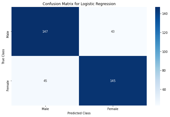
results("Logistic Regression" , log_clf)
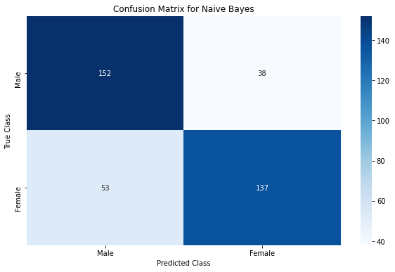
results("Naive Bayes" , nb_clf)
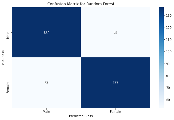
results("Random Forest" , rf_clf)
SVC score: 0.787
              precision    recall  f1-score   support

           0       0.77      0.82      0.79       190
           1       0.80      0.76      0.78       190

    accuracy                           0.79       380
   macro avg       0.79      0.79      0.79       380
weighted avg       0.79      0.79      0.79       380

Logistic Regression score: 0.768
              precision    recall  f1-score   support

           0       0.77      0.77      0.77       190
           1       0.77      0.76      0.77       190

    accuracy                           0.77       380
   macro avg       0.77      0.77      0.77       380
weighted avg       0.77      0.77      0.77       380

Naive Bayes score: 0.761
              precision    recall  f1-score   support

           0       0.74      0.80      0.77       190
           1       0.78      0.72      0.75       190

    accuracy                           0.76       380
   macro avg       0.76      0.76      0.76       380
weighted avg       0.76      0.76      0.76       380

Random Forest score: 0.721
              precision    recall  f1-score   support

           0       0.72      0.72      0.72       190
           1       0.72      0.72      0.72       190

    accuracy                           0.72       380
   macro avg       0.72      0.72      0.72       380
weighted avg       0.72      0.72      0.72       380
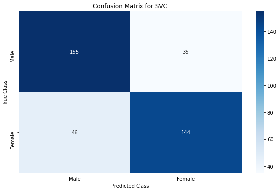
We see that Linear SVC performs the best classification with an accuracy & F1 score of ~79% !!
From the confusion matrix, we can see that out of the 190 male characters in the validation dataset, SVC model classified 155 of them correctly as males, and the remaining 35 incorrectly as females. Similarly, out of 190 female characters in the validation dataset, 144 were classified correctly & 46 classified incorrectly.
Logistic Regression & Naive Bayes classifiers are close at 77% & 76% accuracies respectively. These results are not close to state of the art, but are still pretty good.
Let’s now explore what features contribute the most to our classifiers performance through some model explainability techniques.
Feature importance
Creating a list of all features including numeric, categorical & vectorised features.
vect_columns = list(svc_clf.named_steps['preprocessor'].named_transformers_['vec'].named_steps['tf'].get_feature_names())
onehot_columns = list(svc_clf.named_steps['preprocessor'].named_transformers_['cat'].named_steps['onehot'].get_feature_names(input_features=categorical_features))
numeric_features_list = list(numeric_features)
numeric_features_list.extend(onehot_columns)
numeric_features_list.extend(vect_columns)
Feature importance for Logistic Regression
lr_weights = eli5.explain_weights_df(log_clf.named_steps['classifier'], top=30, feature_names=numeric_features_list)
lr_weights.head(15)
| target | feature | weight | |
|---|---|---|---|
| 0 | 1 | oh | 2.914220 |
| 1 | 1 | really | 1.598428 |
| 2 | 1 | love | 1.582584 |
| 3 | 1 | hi | 1.173297 |
| 4 | 1 | said | 1.161967 |
| 5 | 1 | want | 1.053116 |
| 6 | 1 | like | 1.020965 |
| 7 | 1 | darling | 0.992410 |
| 8 | 1 | never | 0.987203 |
| 9 | 1 | child | 0.975300 |
| 10 | 1 | please | 0.970647 |
| 11 | 1 | god | 0.941234 |
| 12 | 1 | know | 0.913415 |
| 13 | 1 | honey | 0.903731 |
| 14 | 1 | school | 0.897518 |
lr_weights.tail(14)
| target | feature | weight | |
|---|---|---|---|
| 16 | 1 | son | -0.876330 |
| 17 | 1 | good | -0.897884 |
| 18 | 1 | right | -0.899643 |
| 19 | 1 | chId_count | -0.916359 |
| 20 | 1 | fuck | -0.996575 |
| 21 | 1 | fuckin | -1.049543 |
| 22 | 1 | yeah | -1.091158 |
| 23 | 1 | hell | -1.137874 |
| 24 | 1 | got | -1.162604 |
| 25 | 1 | shit | -1.162634 |
| 26 | 1 | sir | -1.201654 |
| 27 | 1 | gotta | -1.246364 |
| 28 | 1 | hey | -1.549047 |
| 29 | 1 | man | -2.188670 |
We see that dialogue keywords like oh, love, like, darling, want, honey are strong indicators that the character is a female, while keywords like son, sir, man, hell, gotta, yeah & most cuss words are usually found in the dialogues of male characters of the given Hollywood movies!
Let’s also try to visualize a single decision tree
We can training a single decision tree using the Random Forest Classifier.
m = RandomForestClassifier(n_estimators=1, min_samples_leaf=5, max_depth = 3,
                           oob_score=True, random_state = np.random.seed(123))
dt_clf = Pipeline(steps=[('preprocessor', preprocessor),
                         ('classifier', m)])

dt_clf.fit(X_train, y_train)
results("Decision Tree Classifier", dt_clf)
Decision Tree Classifier score: 0.526
              precision    recall  f1-score   support

           0       0.54      0.37      0.44       190
           1       0.52      0.68      0.59       190

    accuracy                           0.53       380
   macro avg       0.53      0.53      0.51       380
weighted avg       0.53      0.53      0.51       380
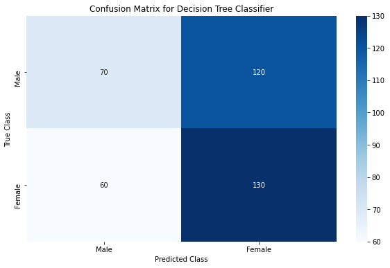
While a single decision is a poor classifier with accuracy barely more than 50%, we see that bagging enough of such weak classifiers to form a Random Forest model helps us improve the model performance drastically! Let’s look at how the splits are made for a single decision tree.
'''
def draw_tree(t, df, size=10, ratio=0.6, precision=0):
    """
    Draws a representation of a decition tree in IPython. Source : fastai v0.7
    Have commented the function definition here due to a Jekyll build error related to Liquid objects.
    """
    s=export_graphviz(t, out_file=None, feature_names=numeric_features_list, filled=True,
                      special_characters=True, rotate=True, precision=precision,
                      proportion=True, class_names = ["male", "female"], impurity = False)
    IPython.display.display(graphviz.Source(re.sub('Tree {',
       f'Tree size={size}; ratio={ratio}', s)))
'''

draw_tree(m.estimators_[0], X_train, precision=2)

Here, the blue coloured nodes indicate their majority class is female while the orange colored nodes have a majority of male labels. The decision tree starts with a mixed sample, but the leaves of the tree are biased towards one class or the other. Most splits seem to be happening using dialogue tokens. For eg., in the above tree, if the tf-idf frequency of keywords think is > 0.1 & kid is > 0.03, the samples are classified as female.
Feature importance for the Random Forest model
eli5.explain_weights_df(rf_clf.named_steps['classifier'], top=30, feature_names=numeric_features_list)
| feature | weight | std | |
|---|---|---|---|
| 0 | oh | 0.077328 | 0.027570 |
| 1 | man | 0.040615 | 0.030255 |
| 2 | love | 0.022664 | 0.026011 |
| 3 | shit | 0.019557 | 0.027031 |
| 4 | said | 0.017135 | 0.018359 |
| 5 | lineLength_median | 0.015757 | 0.017705 |
| 6 | got | 0.013712 | 0.018381 |
| 7 | really | 0.013227 | 0.018366 |
| 8 | hey | 0.012435 | 0.019035 |
| 9 | good | 0.012253 | 0.017000 |
| 10 | look | 0.011174 | 0.016425 |
| 11 | right | 0.009775 | 0.012608 |
| 12 | sir | 0.009673 | 0.018090 |
| 13 | think | 0.009661 | 0.014078 |
| 14 | know | 0.009660 | 0.012629 |
| 15 | em | 0.008794 | 0.019125 |
| 16 | like | 0.008730 | 0.011206 |
| 17 | understand | 0.008263 | 0.013995 |
| 18 | want | 0.008112 | 0.012310 |
| 19 | yeah | 0.007471 | 0.014095 |
| 20 | get | 0.007464 | 0.010990 |
| 21 | would | 0.007399 | 0.010665 |
| 22 | chId_count | 0.007074 | 0.010570 |
| 23 | come | 0.006845 | 0.010507 |
| 24 | god | 0.006782 | 0.011838 |
| 25 | releaseYear | 0.006504 | 0.009230 |
| 26 | hi | 0.006305 | 0.016955 |
| 27 | one | 0.006265 | 0.009646 |
| 28 | gotta | 0.006075 | 0.014320 |
| 29 | child | 0.005858 | 0.013265 |
We see that the median length of a dialogue, total no of lines (chId_count) & movie release year are important features along with the tokens extracted from the character’s dialogues for the Random Forest model!
Next Steps
Some possible ways to further improve the classifier performance could be:
- using bi-grams or tri-grams for dialogue tokens
- Adding features related to sentiments extracted from dialogues
- Adding a feature that measures the level of objectivity or subjectivity of a dialogue
- hyper-parameter tuning of our model parameters
- trying out XGBoost or neural network models
Still, our current best model (Linear SVC) can classify roughly 4 out of 5 movie characters (79% accuracy) correctly using the dialogues they speak, and some movie metadata like release year and position of character in the movie credits. We can safely say that our model is able to capture the gender specific bias in the characters of Hollywood movies.
If you would like to play around with the code, the complete Jupyter notebook is available here on Kaggle.