How matrices transform space

Matrices are objects that operate on vectors

When we mulitply a matrix with an n-dimensional vector, it essentially transforms the vector in n-dimensional space! This wonderful video by 3 Blue 1 Brown expplains this concept through beautiful visualizations - YouTube link

We can take a 2x2 matrix A to consider how it will transform the 2-D space using Python.

import numpy as np
%matplotlib inline
from matplotlib import pyplot

We’ll also need a helper script to plot gridlines in a 2-D space, which we can import from the Github repo of this awesome MOOC.

## Source : https://github.com/engineersCode/EngComp4_landlinear
from urllib.request import urlretrieve
URL = 'https://go.gwu.edu/engcomp4plot'  
urlretrieve(URL, 'plot_helper.py')

('plot_helper.py', <http.client.HTTPMessage at 0x7fc7a1c3f0d0>)

Importing functions (plot_vector, plot_linear_transformation, plot_linear_transformations) from the helper script

from plot_helper import *

Now, let’s take an example of a 2x2 matrix A.

A = np.array([[3, 2],
              [-2, 1]])

Let’s just start with the basis vectors, i_hat and j_hat in 2-D coordinate system, and see how matrix multiplication transforms these 2 basis vectors.

i_hat = np.array([1, 0])
j_hat = np.array([0, 1])

How does the matrix A transform i_hat via multiplication ?

A @ i_hat

array([ 3, -2])

This is just the 1st column of matrix A.

How does the matrix A transform j_hat?

A @ j_hat

array([2, 1])

Similary, multiplication of A with j_hat just gives the second column of matrix A.

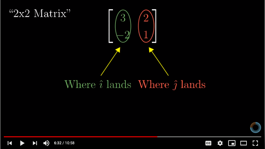
So the columns a matrix, in fact, just give us the location of where our original basis vectors will land. Here’s a screenshot of the above 3B1B video that shows how we can understand this 2-D transformation by simply looking at the columns of the matrix A.

Using our helper script, we can better understand this transformation by looking at the gridlines of our 2-D space before and after transformation.

plot_linear_transformation(A)

Let’s look at another example using another 2x2 matrix M and see how M transforms the 2-D space!

M = np.array([[1,2], [2,1]])
plot_linear_transformation(M)

This also reminds us why “linear algebra” is called “linear”, because A) the origin does not move and B) the gridlines remain parallel straight lines after transformation!

We can now start looking at matrices as not just a collection of numbers in row / column format, but as objects that we can use to transform space the way we want it. And we just need to look at the columns a matrix to understnad where the original basis vectors will land after the transformation!

Here’s another example with the matrix N.

N = np.array([[1,2],[-3,2]])
plot_linear_transformation(N)

Special matrices

Now, let’s look at the some special kinds of matrices. We can rotate the 2-D space by 90 degrees counter clockwise by just rotating the original basis vectors in that direction.

rotation = np.array([[0,-1], [1,0]])
plot_linear_transformation(rotation)

We can even shear the 2-D space by designing our transformation matrix accordingly.

shear = np.array([[1,1], [0,1]])
plot_linear_transformation(shear)

We can scale the X-axis by 2x and Y-axis by 0.5x using the below matrix.

scale = np.array([[2,0], [0,0.5]])
plot_linear_transformation(scale)

Interestingly, we can compose multiple transformations of 2-D space by mulitplying our transformation matrices together. So, applying the above shear and rotation transformations will be the same when done sequentially OR just using the product of the 2 matrices as one single transformation.

plot_linear_transformation(shear@rotation)

plot_linear_transformations(rotation, shear)

However, the order of these transformations is important as matrix multiplication is not commutative!

plot_linear_transformations(shear, rotation)

This concept of space transformation also gives a new meaning to a matrix inverse. The inverse of a matrix simply reverses the transformation of space to its original state.

M = np.array([[1,2], [2,1]])
M_inv = np.linalg.inv(M)
plot_linear_transformations(M, M_inv)

Degenerate matrices will reduce the dimension of the space. For eg, the below matrix D reduces the 2-D space into a 1-D line!

D = np.array([[-2,-1], [1,0.5]])
plot_linear_transformation(D)

Applications in Image Processing

So where can we use this concept of matrix vector multiplication other than in thinking about abstract spaces ? One very important application of this concept can be see in image processing applications. We can consider an image to be a collection of vectors. Let’s consider grayscale images for simplicity, then a grayscale image basically is just a collection of vectors in 2-D space (location of grayscale pixels can be considered a 2-D vector). And we can multiply each pixel vector with a given matrix to transform the entire image!

Let’s import necessary libraries for image manipulation and downloading sample images from the web.

from PIL import Image 
import requests

## Sample image URL
url = 'https://images.pexels.com/photos/2850833/pexels-photo-2850833.jpeg?auto=compress&cs=tinysrgb&dpr=2&h=650&w=940'

Let’s look at our sample image!

im = Image.open(requests.get(url, stream=True).raw)
plt.imshow(im)

<matplotlib.image.AxesImage at 0x7fa0e20d8910>

We will convert this image to grayscale format using the Pillow library.

im = im.convert('LA')
im

Let’s first check the dimensions of our image.

b, h = im.size
b, h

(1300, 1300)

Now, we define a function that will multiply each pixel (2-D vector) of our image with a given matrix.

def linear_transform(trans_mat, b_new = b, h_new = h):
    '''
    Effectively mulitplying each pixel vector by the transformation matrix
    PIL uses a tuple of 1st 2 rows of the inverse matrix
    '''
    Tinv = np.linalg.inv(trans_mat)
    Tinvtuple = (Tinv[0,0],Tinv[0,1], Tinv[0,2], Tinv[1,0],Tinv[1,1],Tinv[1,2])
    return im.transform((int(b_new), int(h_new)), Image.AFFINE, Tinvtuple, resample=Image.BILINEAR) 

Now let’s try scaling our image, 0.25x for X-axis and 0.5x for Y-axis. So our transformation matrix should look like ([0.25, 0], [0, 0.5]). However the Pillow library uses 3x3 matrices rather than a 2x2 matrix. So we can just add the third basis vector to our image without any transformation on it, ie, k_hat.

T = np.matrix([[1/4, 0, 0],
               [0, 1/2, 0],
               [0, 0, 1]])

trans = linear_transform(T, b/4, h/2)
trans

We can rotate our image by 45 degrees counter clockwise using the below matrix.

mat_rotate = (1/ np.sqrt(2)) * \
    np.matrix([[1, -1, 0],
               [1, 1, 0],
               [0, 0, np.sqrt(2)]])

trans = linear_transform(mat_rotate)
trans

After rotation, some pixels move out of our Matplotlib axes frame so we end with a cropped image. We can also combine the scaling and rotation transformations together by using the product of the 2 transformation matrices!

T = mat_rotate @ np.matrix(
    [[1/4, 0, 0],
     [0, 1/4, 0], 
     [0, 0, 1]])

linear_transform(T, b/4, h/4)

I found this idea of matrix vector multiplication very insightful and it’s a pity I never learnt matrix multiplication this was in school or college. If only my school textbooks explained what matrix multiplication actually does rather than just memorizing the formula in a mechanical fashion, I would have really enjoyed learning linear algebra!

If you’re interested to go deep into this topic, I would urge you to check out the YouTube playlist, Essence of Linear Algebra, from 3Blue1Brown. There is also a free MOOC from the George Washington University here and paid one on Coursera available here.

This blog post is written on Jupyter notebooks hosted on Kaggle here and here.

• 2022 2
• 2021 7
• 2020 9